
The Cheapest Cloud Region Is Often the Farthest From Your Users
The same 2 vCPU instance costs $16.23 a month in one region and $39.13 in another — and the cheapest one can be 2.3x slower for your users. A cost-latency reading of 233 cloud regions.
Two spreadsheets landed in the same review last quarter.
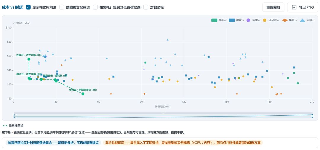
The first came from FinOps. Across 233 cloud regions, the cheapest 2 vCPU / 4 GiB on-demand Linux instance is $5.55 a month.
The second came from the platform team. The region closest to our users answers in 10.7 ms.
Both numbers are right. They point at two places roughly 8,000 km apart.
Nobody made a mistake. Two different questions got squeezed into one meeting, and only one of them was actually about infrastructure.
Price tables have no column for "your users". The cheapest region answers "where is it cheapest to buy" — not "where should this run".
So let's take the three variables in order — price, latency, geography — and see where the single-number answers break.
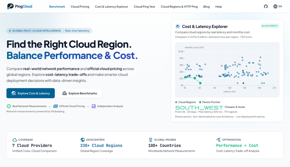
1. Price: the cheapest thing is usually a different thing
The same instance, 2.4x apart
Start with one SKU. Amazon EC2 t4g.medium — 2 vCPU, 4 GiB, ARM, Linux, on-demand — pulled from one official price list:
| Region | Per hour | Per month (730 h) |
|---|---|---|
| Ningxia (cn-northwest-1) | $0.0222 | $16.23 |
| Mumbai / Hyderabad (IN) | $0.0224 | $16.35 |
| N. Virginia (us-east-1) | $0.0336 | $24.53 |
| Frankfurt (eu-central-1) | $0.0384 | $28.03 |
| São Paulo (sa-east-1) | $0.0536 | $39.13 |
Same family, same generation, same specs. Different latitude. 2.4x.
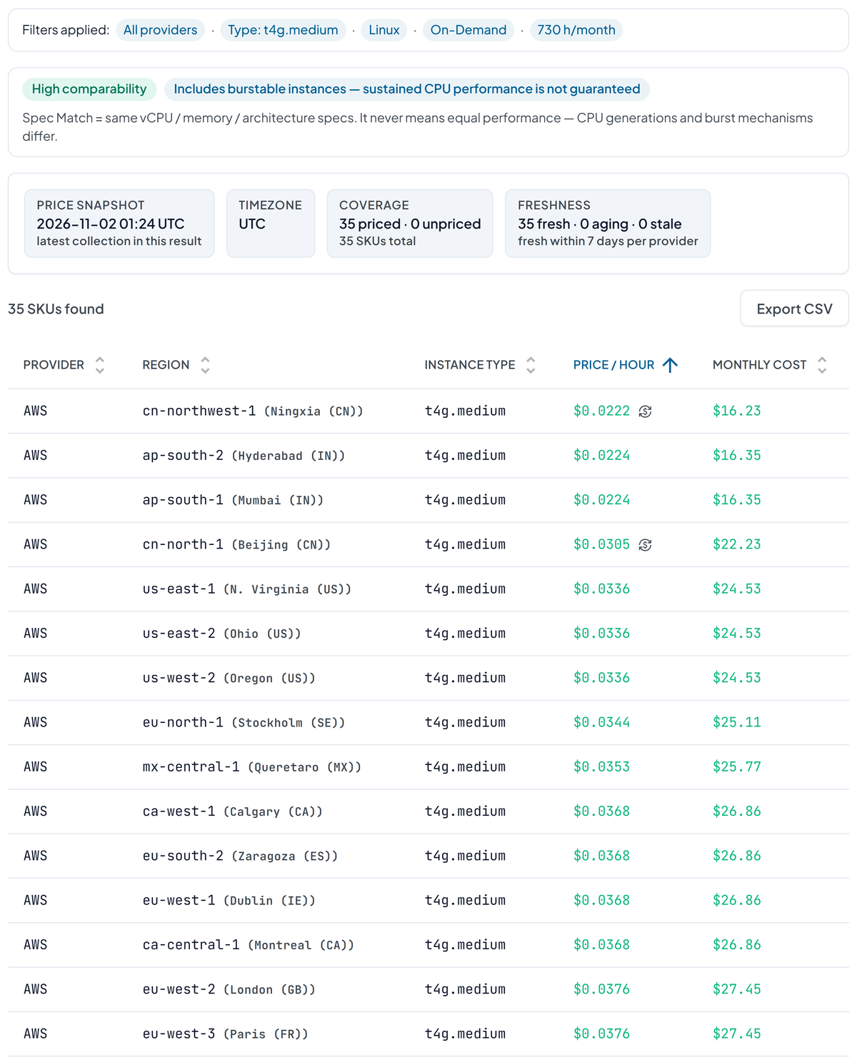
That alone should kill the phrase "the cheapest region". There is no such region — there's only the cheapest region for a given SKU. Change the instance family and the ranking reshuffles.
The same city, 2x apart
Now flip the axis. Pin the vantage point to Germany, keep 2 vCPU / 4 GiB / Linux, and look only at Frankfurt:
| Provider | Instance | Monthly | Avg RTT | Pareto |
|---|---|---|---|---|
| Google Cloud | n4a-highcpu-2 | $55.95 | 10.7 ms | Pareto |
| Tencent Cloud | SA2.MEDIUM4 | $29.20 | 10.8 ms | Pareto |
| AWS | t4g.medium | $28.03 | 11.4 ms | Pareto |
| Alibaba Cloud | ecs.t6-c1m2.large | $29.93 | 11.8 ms | Dominated |
| Azure | Standard_B2pls_v2 | $28.03 | 12.1 ms | Dominated |
Twice the price for 0.7 milliseconds. That is $27.92 a month, per instance, for a difference smaller than a single TCP handshake.
And it is not a measurement artifact: every row here carries 280+ samples from independent probes, all classified high confidence. The gap is real. It is just small — same city, so the fiber run is a few kilometers either way. What differs is peering, the last mile, and how loaded the gateway is at 3 p.m.
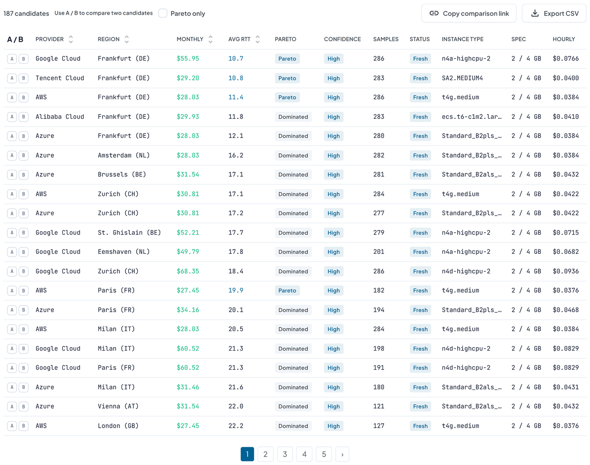
Whether that $27.92 buys you anything is a business question. For a trading gateway it might. For a B2B SaaS with 50,000 daily actives, it almost certainly does not.
"Spec match" is not "performance match"
Underneath both tables sits a quieter trap.
The $28.03 t4g.medium is burstable. The $55.95 n4a-highcpu-2 is dedicated. Both are "2 vCPU / 4 GiB". Their sustained throughput is not in the same league.
Now look at the global floor: the cheapest 2 vCPU / 4 GiB SKUs on PingCloud — Huawei at7.large.2 at $5.55, t7.large.2 at $7.01, Tencent BF1.MEDIUM4, Azure's B series — are all burstable or shared. That is not a coincidence; it is why they are at the floor.
Spec match promises exactly three things: vCPU count, memory in GiB, and CPU architecture. It never promises performance. Burn through the CPU credits and a burstable instance drops to baseline — at which point "cheap" was really "slow", billed monthly.
PingCloud handles this by tagging every comparison with a comparability level (high / medium / low), and by raising a mixed-performance frontier warning inside the explorer whenever the filtered set mixes architectures, burstable and dedicated classes, or different specs. The frontier points then describe a trade-off between unequal things, and the interface says so rather than letting you assume otherwise.
Your price is not the list price
Enterprise discounts, commitments, reserved instances, savings plans, spot. What you actually pay is lower than list, and it is lower by an amount that only you know.
That is precisely why PingCloud collects list prices only. A list price is the one number that is comparable, reproducible and auditable across seven providers. Fold your negotiated rate into a public benchmark and every number in it becomes unfalsifiable.
2. Latency: four traps inside one number
Loss, not just delay
Back to the German vantage point. The $5.55 Huawei Beijing candidate sits at 217.9 ms — and 3.59% packet loss. From the US, the equivalent cheap option (Huawei Guangzhou, $5.55) shows 6.12% loss.
6% loss is not "6% slower". On TCP it means retransmits, congestion windows collapsing, and head-of-line blocking on a single HTTP/2 connection. For API traffic and anything interactive, 6% loss usually hurts more than an extra 20 ms of clean RTT.
An average-only table cannot show you this. PingCloud reports loss next to every latency figure for that reason.
A country aggregate is not your users
Every national number is an aggregate: all measured cities, all probes, weighted by measurement count. Two home broadband lines in the same city can take entirely different submarine routes.
So the explorer ships the sample count, city count and ASN count alongside the average, plus a confidence level. In the Frankfurt table above, AWS shows 286 samples at high confidence. The $5.55 Beijing point that anchors the cheap end of the frontier rests on 13. Both are usable — but only one of them should be the basis of a budget.
Which hop did you measure?
Three tools, three numbers, all correct:
- Browser HTTP ping — a HEAD request from your own network, including DNS, TCP and TLS. Effectively TTFB.
- Cloud ping test — ICMP from a named city's independent probe, single shot.
- Benchmark / explorer — multi-day, multi-city aggregates of 15-packet measurements.
They answer different questions. Using the wrong one is worse than using none — for example, arguing about Southeast Asian user experience with a ping from your office in Frankfurt.
The distribution, not the mean
PingCloud publishes average, median and P95 per candidate, and is explicit about one limit: P95 at the packet level would require storing raw per-packet timings, which the system does not. So it reports P95 of per-measurement medians, and labels it as such. It does not estimate the rest.
That kind of restraint is rarer than it should be, and it matters when you are about to sign a three-year commitment based on a chart.
3. The marginal cost of a millisecond is not linear
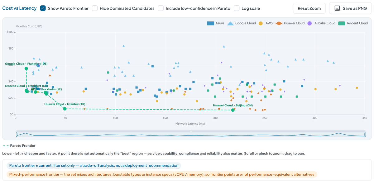
Plot the 187 German-vantage candidates on cost × latency and the Pareto frontier collapses to 8 points:
| Region | Monthly | Avg RTT | Cost of the step |
|---|---|---|---|
| Huawei Cloud Beijing | $5.55 | 217.9 ms | — |
| Huawei Cloud Istanbul | $7.01 | 49.4 ms | +$1.46 for −168.5 ms → $0.009/ms |
| AWS Stockholm | $25.11 | 30.9 ms | +$18.10 for −18.5 ms → $0.98/ms |
| AWS Dublin | $26.86 | 30.0 ms | +$1.75 for −0.9 ms → $1.88/ms |
| AWS Paris | $27.45 | 19.9 ms | +$0.58 for −10.1 ms → $0.058/ms |
| AWS Frankfurt | $28.03 | 11.4 ms | +$0.58 for −8.5 ms → $0.069/ms |
| Tencent Cloud Frankfurt | $29.20 | 10.8 ms | +$1.17 for −0.6 ms → $1.95/ms |
| Google Cloud Frankfurt | $55.95 | 10.7 ms | +$26.75 for −0.1 ms → $243/ms |
Read it as a price list for milliseconds.
The first step is the best deal on the internet: $1.46 buys back 168 milliseconds. Nine-tenths of a cent per millisecond.
The middle is still sane: $21 takes you from 49 ms to 11.4 ms.
Then it breaks. The final step — Tencent Frankfurt to Google Frankfurt — costs $26.75 to save 0.11 ms. At $243 per millisecond, it is 125x more expensive than the step immediately before it.
Notice also the Dublin row: $1.75 for 0.93 ms. The frontier is not a ladder with a smooth gradient; it is a shape. Some points on it are outright bad deals that survive only because nothing else occupies that exact position.
4. Geography changes the frontier itself
Here is the part that a price table can never tell you: the frontier is a function of where your users are.
Run the same query — 2 vCPU / 4 GiB, 720-hour window — from four vantage points:
| Users in | Frontier points | Cheapest on frontier | Fastest available |
|---|---|---|---|
| Germany | 8 | $5.55 · 217.9 ms | $55.95 · 10.7 ms |
| United States | 4 | $5.55 · 218.1 ms | $24.53 · 31.3 ms |
| Japan | 6 | $5.55 · 153.6 ms | $31.75 · 12.9 ms |
| Brazil | 2 | $7.01 · 22.0 ms | $43.80 · 21.9 ms |
Four different option sets, from one spec sheet.
In Japan, six options survive and the trade is honest: Huawei Hong Kong at $5.99 delivers 67.3 ms, AWS Osaka at $31.75 delivers 12.9 ms. 5.3x the price for 5.2x less latency. If Tokyo is your core market, that is a fair trade — take it.
In Brazil, the frontier shrinks to two points and both are in São Paulo. The $5.55 Chinese SKU is still cheaper on paper, but it is 354 ms away and too thinly sampled to clear the confidence bar, so it never enters the frontier at all. The real decision is $7.01 Huawei São Paulo (22.0 ms) versus $43.80 Tencent São Paulo (21.9 ms) — 6.2x the price for 0.14 ms. That one you decline without a meeting.
And the headline arithmetic: the same $5.55 SKU, unchanged, reads 153.6 ms from Tokyo, 217.9 ms from Frankfurt, 354.3 ms from São Paulo. 2.3x, with the price tag nailed to the wall.
"Cheapest" is an absolute claim. "How far is it from my users" is a relative one. The price table sorts by dollars; your users are distributed by longitude.
5. Pareto, and where it stops
Candidate A dominates candidate B when A costs no more and is no slower, with at least one strict improvement. The frontier is everything not dominated — and in a 187-candidate field, that is 8 rows worth of attention.
Three caveats the interface states outright, because they matter:
- The frontier is not a recommendation. It optimises two objectives. Compliance, data residency, service availability in that region, SLA, AZ count, and cross-region egress costs are all outside the plot.
- A mixed-performance frontier is not comparable. If burstable and dedicated instances share a filter set, the points do not trade off like for like.
- Low-confidence candidates stay out by default. Thin samples are shown, flagged, and excluded from the frontier rather than silently averaged in.

That card is the whole problem in one line: three different "bests" in three different places.
6. How the numbers are produced
Three rules, each of which costs the platform something to keep.
Probes outside the providers' own networks. Measurements run on the Globalping volunteer network — 1,053 active probe cities across 113 countries, roughly 4,900 available probes, sitting in real homes, offices and ISP networks. Probes hosted on the seven measured providers' own infrastructure are excluded at three layers. Before that exclusion, provider-hosted probes decided the winner in 8 countries on the 7-day leaderboard — every probe in Chuncheon, South Korea sat on Oracle's network, which measured Oracle at 10.0 ms ahead of Azure Seoul at 11.9 ms from independent networks. No provider grades its own exam.
Official prices only, no estimation. AWS Bulk Price List API, Azure Retail Prices API, Google Cloud Billing Catalog, Alibaba's calculator API, Tencent's CVM gateway, Huawei's calculator cross-checked against BSS, OCI's cost estimator. Synced weekly, flagged past seven days. Currently 192,466 region-level compute SKUs. Where an official machine-readable price does not exist — Huawei spot pricing, OCI GPU SKUs that cannot be split from the GPU part — the row is absent rather than approximated.
Same probe, same parameters, same cycle. Within a cycle, one probe measures every provider's regions with identical settings. 15 ICMP packets per measurement, medians from raw samples, aggregation weighted by measurement count, cities above 50% loss dropped. Fairness here is a property of the pipeline, not a claim in a footnote.
The rankings, API and monthly archives are public and free to cite.
7. Six steps that survive contact with a budget
- Map your users by country. From analytics, not intuition. This sets the denominator for everything else.
- Shortlist with the benchmark. The top 10–20 regions by weighted median latency for each country where you actually have users.
- Fix the spec, then read the frontier. vCPU, memory, architecture, and CPU performance model locked — otherwise you are comparing unlike things.
- Price the milliseconds. Compute the marginal cost of each step on the frontier. Stop where it leaves your value range.
- Verify the live path. Peering changes. Run a cloud ping test from the target city, then load-test the real workload.
- Prune with hard constraints. Compliance, service catalogue, SLA, AZ count, migration cost. A region that fails compliance does not exist, however fast it is.
Order matters: prune first, optimise second. Reversed, you will spend a week optimising a region you cannot legally use.
The cheapest cloud region is often the farthest from your users — not because the prices are wrong, but because a price table has no column for distance. One dimension of data cannot answer a two-dimensional question, and the missing dimension is always the same one: where are the people?
Try it on your own numbers: Cost & Latency Explorer — pick a source country, set the spec, read the frontier. No account required. Methodology and the free API are documented in the Help Center.